Flow chart
If either Numba or JAX have enough feature to acommplish what you need, performance-wise, here’s a flowchart:

Research Software & Analytics Group, University of Exeter
September 21st, 2025
Languages that has demonstrated to scale to state-of-the-art, full system supercomputer
gcc from GNU compilers, clang from LLVM
compilers
pypypypy: general purpose Python implementation (any valid
Python should runs)To replace this single function from Numba to C++ with pybind11,
@numba.jit(parallel=True)
def _fma(out, weights, *arrays):
    for weight, array in zip(weights, arrays):
out += weight * array14 files changed
+230 -36 lines changed… and 30% faster!
Python gives you velocity: rapid prototyping science code is a path dependent evolution
Numba jit gives you speed (SIMD + multi-threading): C++ with SIMD
and OpenMP multi-threading is only 30% faster in this case. The single
@jit decorator gives you 3 times speed up comparing to pure
Numpy implementation.
JIT sometimes has advantage over AOT because it can see the data
JIT obviously has overhead, but if you are processing “big data”, that amount of time usually is much shorter than it takes to run the calculation itself.
\[\tilde{w}_{ij} = \sum_{k=1}^K \frac{1}{n_k^2} \cos \left( 2 \pi \left[ \left(\vec{g}_i - \vec{g}_j \right) \cdot \vec{u}_k \right] \right) ,\quad 1 \leq i, j \leq M\]
\[\tilde{w}_{ij} = \sum_{k=1}^K \frac{1}{n_k^2} \cos \left( 2 \pi \left[ \left(\vec{g}_i - \vec{g}_j \right) \cdot \vec{u}_k \right] \right) ,\quad 1 \leq i, j \leq M\]
As usual in Numpy, we vectorize everything:
import numpy as np


def w_mm_np(
    n_k: np.ndarray[tuple[int], np.float64],
    u_k_vec: np.ndarray[tuple[int, int], np.float64],
    g_m_vec: np.ndarray[tuple[int, int], np.float64],
) -> np.ndarray[tuple[int, int], np.float64]:
    # (M, M, 1, 2)
    δg_mm1_vec =  g_m_vec.reshape(-1, 1, 1, 2) - g_m_vec.reshape(1, -1, 1, 2)
    # (1, 1, K, 2)
    u_11k_vec = u_k_vec.reshape(1, 1, -1, 2)
    return (
        np.cos(
            (2.0 * np.pi) *
            # (M, M, K)
            (
                δg_mm1_vec[:, :, :, 0] * u_11k_vec[:, :, :, 1] +
                δg_mm1_vec[:, :, :, 1] * u_11k_vec[:, :, :, 0]
            )
        ) /
        # (1, 1, K)
        np.square(n_k).reshape(1, 1, -1)
    ).sum(2)  # sum over k
898 ms ± 9.62 ms per loop (mean ± std. dev. of 7 runs, 1 loop each)How would you implement it in Numba? Just add the jit decorator:
import numba


@numba.jit("f8[:, ::1](f8[::1], f8[:, ::1], f8[:, ::1])", nopython=True, nogil=True, parallel=True)
def w_mm_numba(
    ...
522 ms ± 9.01 ms per loop (mean ± std. dev. of 7 runs, 1 loop each)How would you implement it in JAX? By add the jit decorator, and
replacing numpy with jax.numpy:
import jax
import jax.numpy as jnp

@jax.jit
def w_mm_jax(
    n_k: np.ndarray[tuple[int], np.float64],
    u_k_vec: np.ndarray[tuple[int, int], np.float64],
    g_m_vec: np.ndarray[tuple[int, int], np.float64],
) -> np.ndarray[tuple[int, int], np.float64]:
    # (M, M, 1, 2)
    δg_mm1_vec =  g_m_vec.reshape(-1, 1, 1, 2) - g_m_vec.reshape(1, -1, 1, 2)
    # (1, 1, K, 2)
    u_11k_vec = u_k_vec.reshape(1, 1, -1, 2)
    return (
        jnp.cos(
            (2.0 * jnp.pi) *
            # (M, M, K)
            (
                δg_mm1_vec[:, :, :, 0] * u_11k_vec[:, :, :, 1] +
                δg_mm1_vec[:, :, :, 1] * u_11k_vec[:, :, :, 0]
            )
        ) /
        # (1, 1, K)
        jnp.square(n_k).reshape(1, 1, -1)
    ).sum(2)  # sum over k
144 ms ± 1.53 ms per loop (mean ± std. dev. of 7 runs, 10 loops each)import numpy as np
def w_mm_np(
n_k: np.ndarray[tuple[int], np.float64],
u_k_vec: np.ndarray[tuple[int, int], np.float64],
g_m_vec: np.ndarray[tuple[int, int], np.float64],
) -> np.ndarray[tuple[int, int], np.float64]:
# (M, M, 1, 2)
δg_mm1_vec = g_m_vec.reshape(-1, 1, 1, 2) - g_m_vec.reshape(1, -1, 1, 2)
# (1, 1, K, 2)
u_11k_vec = u_k_vec.reshape(1, 1, -1, 2)
return (
np.cos(
(2.0 * np.pi) *
# (M, M, K)
(
δg_mm1_vec[:, :, :, 0] * u_11k_vec[:, :, :, 1] +
δg_mm1_vec[:, :, :, 1] * u_11k_vec[:, :, :, 0]
)
) /
# (1, 1, K)
np.square(n_k).reshape(1, 1, -1)
).sum(2) # sum over k\[\tilde{w}_{ij} = \sum_{k=1}^K \frac{1}{n_k^2} \cos \left( 2 \pi \left[ \left(\vec{g}_i - \vec{g}_j \right) \cdot \vec{u}_k \right] \right) ,\quad 1 \leq i, j \leq M\]
\((M, M, K, 2)\) of 64-bit array would be \(\sim 700\) PiB!
While \((M, M)\) of 64-bit array would be \(\sim 40\) GiB only.
To put that into perspective, whole system aggregated memory of NERSC is \(\sim 2\text{ PiB}\).
@numba.jit("f8[:, ::1](f8[::1], f8[:, ::1], f8[:, ::1])", nopython=True, nogil=True, parallel=True)
def w_mm_numba_iterative(
    n_k: np.ndarray[tuple[int], np.float64],
    u_k_vec: np.ndarray[tuple[int, int], np.float64],
    g_m_vec: np.ndarray[tuple[int, int], np.float64],
) -> np.ndarray[tuple[int, int], np.float64]:
    M = g_m_vec.shape[0]
    K = u_k_vec.shape[0]
    δg_mm_vec = g_m_vec.reshape(-1, 1, 2) - g_m_vec.reshape(1, -1, 2)

    w_mm = np.zeros((M, M))
    for k in numba.prange(K):
        w_mm += np.cos((2.0 * np.pi) * (δg_mm_vec[:, :, 1] * u_k_vec[k, 0] + δg_mm_vec[:, :, 0] * u_k_vec[k, 1])) / np.square(n_k[k])
    return w_mm
55 ms ± 1.59 ms per loop (mean ± std. dev. of 7 runs, 10 loops each)@jax.jit
def w_mm_jax_iterative(
n_k: np.ndarray[tuple[int], np.float64],
u_k_vec: np.ndarray[tuple[int, int], np.float64],
g_m_vec: np.ndarray[tuple[int, int], np.float64],
) -> np.ndarray[tuple[int, int], np.float64]:
M = g_m_vec.shape[0]
δg_mm_vec = g_m_vec.reshape(M, 1, 2) - g_m_vec.reshape(1, M, 2)
δg_mm_y = δg_mm_vec[:, :, 0]
δg_mm_x = δg_mm_vec[:, :, 1]
def _w_mm_k(
n: float,
u_vec: np.ndarray[tuple[int], np.float64],
) -> np.ndarray[tuple[int, int], np.float64]:
return jnp.cos((2.0 * jnp.pi) * (δg_mm_x * u_vec[0] + δg_mm_y * u_vec[1])) / (n * n)
def _accumulate_w_mm(
sum_: np.ndarray[tuple[int, int], np.float64],
args: tuple[float, np.ndarray[tuple[int], np.float64]],
) -> tuple[np.ndarray[tuple[int, int], np.float64], None]:
n, u_vec = args
return sum_ + _w_mm_k(n, u_vec), None
res, _ = jax.lax.scan(
_accumulate_w_mm,
jnp.zeros((M, M)),
(
n_k,
u_k_vec,
),
)
return res86.6 ms ± 102 μs per loop (mean ± std. dev. of 7 runs, 10 loops each)numba.cuda is an entirely different interface| Numba | JAX |
|---|---|
| C-like mini language | Smaller language (\(\text{JAX} \underset{\sim}{\subset} \text{Numba}\)): restrictions on control flow, mutation, and dynamic shapes |
| Implements a subset of Python+NumPy, with a parallelization model similar to a mini-“OpenMP” | Implements a subset of Python+NumPy+SciPy exposed via duck-typing. |
| NumPy implementations are dropped in replacement but only a subset is implemented. Calling NumPy within jitted function is completely hijacked. Documentation is minimal. | jax.numpy
and jax.scipy
have similar API comparing to NumPy and SciPy, but has its own
documentation. This facilitates deviations
in behaviors. |
| Functions “recompile” whenever input type changes. | Functions “recompile” whenever input type and shape changes. |
| No automatic compiling & offloading to accelerator. No autograd/autodiff. | Going through FFI is more costly: memory transfer from and to device, losing autograd/autodiff. |
tracing compiler & recompile per shape change \(\Rightarrow\)
static_argnums
Compiler Driven Design
Easy to port to GPU without setting one up.
JAX vs numba-cuda: The XLA compiler handles device-specific optimization automatically.
As a functional language, JAX nudges you to write correct code, and performance comes as a bonus.
\[\tilde{w}_{ij} = \sum_{k=1}^K \frac{1}{n_k^2} \cos \left( 2 \pi \left[ \left(\vec{g}_i - \vec{g}_j \right) \cdot \vec{u}_k \right] \right) ,\quad 1 \leq i, j \leq M\]
| Implementation | s | σ |
|---|---|---|
jax_compact |
2.5543 (1.00) | 0.0050 |
numba_compact |
2.8768 (1.13) | 0.0012 |
jax |
3,368.6229 (>1000.0) | 1.6803 |
numba |
3,702.7006 (>1000.0) | 0.7385 |
| Implementation | ms | σ |
|---|---|---|
numba_compact |
2.5029 (1.0) | 0.0520 |
jax_compact |
61.5560 (24.59) | 6.8555 |
jax |
143.2451 (57.23) | 0.0749 |
numba |
1,794.1949 (716.83) | 14.9648 |
\[F = T^T \tilde{w} T\]
| Implementation | ms | σ |
|---|---|---|
numba_sparse |
8.0733 (1.0) | 0.0501 |
jax |
19.7302 (2.44) | 1.6986 |
jax_sparse |
25.0091 (3.10) | 0.1484 |
jax_BCOO |
48.5340 (6.01) | 0.1571 |
numba_compact_sparse |
49.8400 (6.17) | 0.0794 |
original_preload_direct |
99.2061 (12.29) | 0.3163 |
numba |
125.3019 (15.52) | 0.1143 |
original |
132.4863 (16.41) | 0.1376 |
numba_compact_sparse_direct |
139.9244 (17.33) | 0.1562 |
jax_compact_sparse_BCOO |
379.7214 (47.03) | 1.4144 |
jax_compact_sparse |
380.8865 (47.18) | 2.4322 |
| Implementation | μs | σ |
|---|---|---|
jax |
260.5957 (1.0) | 29.3714 |
jax_BCOO |
3,078.2068 (11.81) | 35.9463 |
jax_compact_sparse_BCOO |
3,207.3388 (12.31) | 107.0798 |
numba_sparse |
5,548.5175 (21.29) | 64.3711 |
jax_compact_sparse |
7,190.9015 (27.59) | 35.7355 |
numba |
18,187.5003 (69.79) | 5,603.6081 |
original |
18,279.9851 (70.15) | 6,052.1386 |
jax_sparse |
19,786.7200 (75.93) | 42.9344 |
numba_compact_sparse |
32,605.2243 (125.12) | 248.8764 |
numba_compact_sparse_direct |
1,362,329.9249 (>1000.0) | 1,366.9112 |
original_preload_direct |
25,218,633.7856 (>1000.0) | 8,722.4870 |
If either Numba or JAX have enough feature to acommplish what you need, performance-wise, here’s a flowchart:

jax.grad)
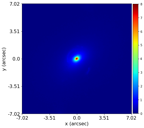
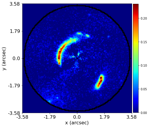
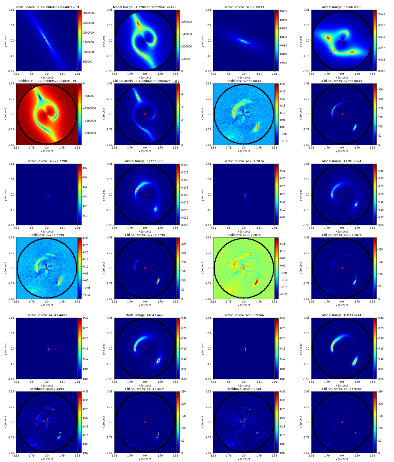
PyAutoLens (via PyAutoFit) supports Nested sampling (Dynesty), MCMC (emcee), particle swarm optimization (PySwarms)


PyAutoLens (via PyAutoFit) supports Nested sampling (Dynesty), MCMC (emcee), particle swarm optimization (PySwarms)
