Physics: revealing the nature of dark matter with the James Webb Space Telescope (JWST)

• Probing the low-mass region (\(\lesssim 10^{8.5} M_\odot\)) of Dark Matter substructures
  • ΛCDM vs. alternative Dark Matter models
  • invisible \(\Rightarrow\) probing via strong gravitational lensing
  • demonstrated in Nightingale et al. (2023) using Hubble Space Telescope (HST) data
• Next: take advantage of 4+ wavebands, high quality observations from James Webb Space Telescope (JWST)

How? PyAutoLens

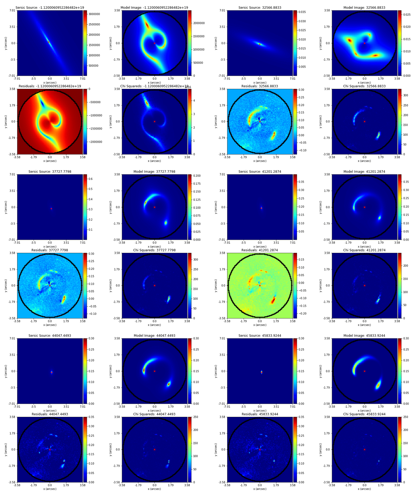
1. Mass modeling: parametric, non-linear, multi-phase models

2. Source reconstruction: linear, reconstructing unlensed light distribution via different kinds of meshes: rectangular, Delaunay, Voronoi

Log-likelihood function takes the output of (1) and computes its likelihood (where (2) is part of the calculation).

Key goal is to automate the whole process and apply it to large datasets.

The power of likelihood in theory

\(P(\boldsymbol{\Theta} | \mathbf{D}, M) = \frac{P(\mathbf{D} | \boldsymbol{\Theta}, M) P(\boldsymbol{\Theta} | M)}{P(\mathbf{D} | M)} \equiv \frac{\mathcal{L}(\boldsymbol{\Theta}) \pi(\boldsymbol{\Theta})} {\mathcal{Z}}\)

The power of likelihood in action

The power of likelihood in action

Computational challenges

• PyAutoLens originally is implemented in Numba
• For single-band HST data, the image processing analysis of a single lens takes approximately 48 hours over 76 CPUs.
  • image pixels: \(M \sim 10,000\)
  • source image pixels: \(S \sim 2,000\)
  • \(3\text{ s}\) for 1 iteration, \(O(100,000)\) iterations needed.
• For JWST’s 4x freq. bands, \(M \rightarrow 4M, S \rightarrow 4S\). Runtime: \(\sim 3\text{ s} \rightarrow 60\text{ s}\). I.e. \(\sim \times 20\)

Why JAX?

• Herculens (Galan et al. 2022), GIGA-Lens (Gu et al. 2022) demonstrated successful adoption of JAX in modeling strong gravitational lensing.
• Performance gains potentially come from:
  • Functions implemented with JAX become faster
  • Running on accelerators
  • Gradient information reduces no. of iterations in fitting
• This project ports the likelihood function, a subset of functionality provided in PyAutoLens, from Numba to JAX

Methodology

• Porting
  1. translate the function to Math
  2. translate the Math to Numba, using vectorized programming as much as possible to anticipate the programming paradigm in JAX
  3. translate the Numba function to JAX, where in simple case would just work
  4. further optimize from there
• Organizing & Testing
  • Functions are then kept in 3 different modules, original for the original functions, numba for those ported in (2), jax for those ported in (3)
  • Metaprogramming is used in setting up unit-test framework (via pytest) to guarantee correctness. pytest-benchmark is used to compare performance differences between these implementations. This feeds back into step (4).

What is Numba

• Numba is a jit compiler supporting a subset of Python and NumPy operations, powered by LLVM. While it is possible to target the GPU via CUDA, it requires rewriting the function using different APIs and paradigms, not to mention it is CUDA (i.e. NVidia) only.

What is JAX

• JAX is a jit compiler, tracing compiler by Google, powered by XLA compiler, originated from Google. JAX is designed primarily for machine learning workloads but is suitable for scientific computing as well. It is a tracing compiler removing side-effects of function. I.e. effectively it encourages functional programming paradigm and thinking. It automatically targets multiple hardware architectures including CPU, GPU, TPU, without requiring rewriting.
• I.e. it solves the “two-language problem”, or more accurately, “three-implementation problem”: prototype/API, CPU, GPU.

Numba vs. JAX

Characteristics of JAX

• tracing compiler & recompile per shape change \(\Rightarrow\) static_argnums

  @partial(jax.jit, static_argnums=0)
  def this_recompile_everytime(shape):
      return jax.numpy.zeros(shape)

• Compiler Driven Design

  • Especially in JAX, partly because of its functional paradigm, framing your problem in JAX idiomatic expressions results in great speed up, sometimes more than you could do otherwise in Numba because of its design (recompile per shape, fusion/fusing compatible operations, etc.), but you’ll hit a wall if you want more low-level optimizations.
  • It can also means performance improvements can come for free through compiler improvements, as long as your code is written in JAX idiomatic way.

• Easy to port to GPU without setting one up.

• JAX vs numba-cuda: The XLA compiler handles device-specific optimization automatically.

• JAX nudges you to write correct code, and performance comes as a bonus.

\(\tilde{w}\)—Code: original version

\[\tilde{W}_{ij} = \sum_{k=1}^K \frac{1}{n_k^2} \cos(2\pi[(g_{i1} - g_{j1})u_{k0} + (g_{i0} - g_{j0})u_{k1}])\]

@numba.jit(nopython=True, nogil=True, parallel=True)
def w_tilde_curvature_interferometer_from(
    noise_map_real: np.ndarray,
    uv_wavelengths: np.ndarray,
    grid_radians_slim: np.ndarray,
) -> np.ndarray:
    w_tilde = np.zeros((grid_radians_slim.shape[0], grid_radians_slim.shape[0]))

    for i in range(w_tilde.shape[0]):
        for j in range(i, w_tilde.shape[1]):
            y_offset = grid_radians_slim[i, 1] - grid_radians_slim[j, 1]
            x_offset = grid_radians_slim[i, 0] - grid_radians_slim[j, 0]

            for vis_1d_index in range(uv_wavelengths.shape[0]):
                w_tilde[i, j] += noise_map_real[vis_1d_index] ** -2.0 * np.cos(
                    2.0
                    * np.pi
                    * (y_offset * uv_wavelengths[vis_1d_index, 0] + x_offset * uv_wavelengths[vis_1d_index, 1])
                )

    for i in range(w_tilde.shape[0]):
        for j in range(i, w_tilde.shape[1]):
            w_tilde[j, i] = w_tilde[i, j]

    return w_tilde

\(\tilde{w}\)—Code: 1st try

\[\tilde{W}_{ij} = \sum_{k=1}^K \frac{1}{n_k^2} \cos(2\pi[(g_{i1} - g_{j1})u_{k0} + (g_{i0} - g_{j0})u_{k1}])\]

@jax.jit
def w_tilde_curvature_interferometer_from(
    noise_map_real: np.ndarray[tuple[int], np.float64],
    uv_wavelengths: np.ndarray[tuple[int, int], np.float64],
    grid_radians_slim: np.ndarray[tuple[int, int], np.float64],
) -> np.ndarray[tuple[int, int], np.float64]:
    # (M, M, 1, 2)
    g_ij =  grid_radians_slim.reshape(-1, 1, 1, 2) - grid_radians_slim.reshape(1, -1, 1, 2)
    # (1, 1, K, 2)
    u_k = uv_wavelengths.reshape(1, 1, -1, 2)
    return (
        jnp.cos(
            (2.0 * jnp.pi) *
            # (M, M, K)
            (
                g_ij[:, :, :, 0] * u_k[:, :, :, 1] +
                g_ij[:, :, :, 1] * u_k[:, :, :, 0]
            )
        ) /
        # (1, 1, K)
        jnp.square(noise_map_real).reshape(1, 1, -1)
    ).sum(2)  # sum over k

\(\tilde{w}\)—Code: 2nd try

\[\tilde{W}_{ij} = \sum_{k=1}^K \frac{1}{n_k^2} \cos(2\pi[(g_{i1} - g_{j1})u_{k0} + (g_{i0} - g_{j0})u_{k1}])\]

@jax.jit
def w_tilde_curvature_interferometer_from(
    noise_map_real: np.ndarray[tuple[int], np.float64],
    uv_wavelengths: np.ndarray[tuple[int, int], np.float64],
    grid_radians_slim: np.ndarray[tuple[int, int], np.float64],
) -> np.ndarray[tuple[int, int], np.float64]:
    # A_mk, m<M, k<K
    # assume M > K to put TWO_PI multiplication there
    A = grid_radians_slim @ (TWO_PI * uv_wavelengths)[:, ::-1].T

    noise_map_real_inv = jnp.reciprocal(noise_map_real)
    C = jnp.cos(A) * noise_map_real_inv
    S = jnp.sin(A) * noise_map_real_inv

    return C @ C.T + S @ S.T

\(\tilde{w}\)—Code: digression in problem sizes

\[\tilde{W}_{ij} = \sum_{k=1}^K \frac{1}{n_k^2} \cos(2\pi[(g_{i1} - g_{j1})u_{k0} + (g_{i0} - g_{j0})u_{k1}])\]

Number of image pixels

\(M \sim 70,000 \Rightarrow M^2 \sim 5 \times 10^9, \quad 0 \leq i, j < M\)

\(N \sim \sqrt{M} \sim 300\)

Number of visibilities

\(K \sim 10^7, \quad 0 \leq k < K\)

\((M, M, K, 2)\) of 64-bit array would be \(\sim 700\) PiB!

While \((M, M)\) of 64-bit array would be \(\sim 40\) GiB only.

\(\tilde{w}\)—Code: final try—Numba

\[\tilde{W}_{ij} = \sum_{k=1}^K \frac{1}{n_k^2} \cos(2\pi[(g_{i1} - g_{j1})u_{k0} + (g_{i0} - g_{j0})u_{k1}])\]

@numba.jit("f8[:, ::1](f8[::1], f8[:, ::1], f8[:, ::1])", nopython=True, nogil=True, parallel=True)
def w_tilde_curvature_interferometer_from(
    noise_map_real: np.ndarray[tuple[int], np.float64],
    uv_wavelengths: np.ndarray[tuple[int, int], np.float64],
    grid_radians_slim: np.ndarray[tuple[int, int], np.float64],
) -> np.ndarray[tuple[int, int], np.float64]:
    M = grid_radians_slim.shape[0]
    K = uv_wavelengths.shape[0]
    g_2pi = TWO_PI * grid_radians_slim
    δg_2pi = g_2pi.reshape(-1, 1, 2) - g_2pi.reshape(1, -1, 2)

    w = np.zeros((M, M))
    for k in numba.prange(K):
        w += np.cos(δg_2pi[:, :, 1] * uv_wavelengths[k, 0] + δg_2pi[:, :, 0] * uv_wavelengths[k, 1]) * np.reciprocal(
            np.square(noise_map_real[k])
        )
    return w

\(\tilde{w}\)—Code: final try—JAX

@jax.jit
def w_tilde_curvature_interferometer_from(
    noise_map_real: np.ndarray[tuple[int], np.float64],
    uv_wavelengths: np.ndarray[tuple[int, int], np.float64],
    grid_radians_slim: np.ndarray[tuple[int, int], np.float64],
) -> np.ndarray[tuple[int, int], np.float64]:
    M = grid_radians_slim.shape[0]
    g_2pi = TWO_PI * grid_radians_slim
    δg_2pi = g_2pi.reshape(M, 1, 2) - g_2pi.reshape(1, M, 2)
    δg_2pi_y = δg_2pi[:, :, 0]
    δg_2pi_x = δg_2pi[:, :, 1]

    def f_k(
        noise_map_real: float,
        uv_wavelengths: np.ndarray[tuple[int], np.float64],
    ) -> np.ndarray[tuple[int, int], np.float64]:
        return jnp.cos(δg_2pi_x * uv_wavelengths[0] + δg_2pi_y * uv_wavelengths[1]) * jnp.reciprocal(
            jnp.square(noise_map_real)
        )

    def f_scan(
        sum_: np.ndarray[tuple[int, int], np.float64],
        args: tuple[float, np.ndarray[tuple[int], np.float64]],
    ) -> tuple[np.ndarray[tuple[int, int], np.float64], None]:
        noise_map_real, uv_wavelengths = args
        return sum_ + f_k(noise_map_real, uv_wavelengths), None

    res, _ = jax.lax.scan(
        f_scan,
        jnp.zeros((M, M)),
        (
            noise_map_real,
            uv_wavelengths,
        ),
    )
    return res

Match 1: Numba vs JAX with 1 CPU core

Match 2: Numba with 128 CPU cores and JAX with CUDA on GPU (A100)

Bonus round 1: Numba vs JAX with 1 CPU core (\(F\))

\[F = T^T \tilde{w} T\]

Bonus round 2: Numba with 128 CPU cores and JAX with CUDA on GPU (A100) (\(F\))

Takeaway from benchmark analysis

• “Porting Numba to Numba” is faster in many cases
• The only fair fight between Numba and JAX is single CPU core benchmark
• Different algorithms of the same function is faster (even across Numba and JAX) depending on input sizes
  • \(\Rightarrow\) keep all implementations \(\rightarrow\) profile \(\rightarrow\) pick best (per science case per system)

Limitation of JAX on CPU

• JAX for multithreading on the CPU is a rabbit hole. All links below are from GitHub issues. The lack of documentation reflects on the lack of interest in multicore parallelism on the CPU from the primarily machine learning community (JAX from Google, XLA from OpenXLA).

  From JAX running in CPU only mode only uses a single core:

  This is largely working as intended at the moment. JAX doesn’t parallelize operations across CPU cores unless you use explicit parallelism constructs like pmap. Some JAX operations (e.g., BLAS or LAPACK) operations have their own internal parallelism.

• In an HPC setting, you may want to use multiple hierarchies of parallelism on the CPU: SIMD + Multi-threading (e.g. OpenMP) + Multi-processing (e.g. MPI). In this case, you’d want to limit the number of CPU cores for multi-threading, often set via ..._NUM_THREADS. This is very obscure in how to achieve such in JAX:

  • XLA_FLAGS='--xla_cpu_multi_thread_eigen=false intra_op_parallelism_threads=1' was the recommendation. It is now recommended to use NPROC=1 to disable multithreading used in Eigen instead. Notice the lack of JAX_NUM_THREADS \(\Rightarrow\) NPROC might have side-effects.

  export MKL_NUM_THREADS=${NUM_THREADS}
  export MKL_DOMAIN_NUM_THREADS="MKL_BLAS=${NUM_THREADS}"
  export MKL_DYNAMIC=FALSE
  
  export OMP_NUM_THREADS=${NUM_THREADS}
  export OMP_PLACES=threads
  export OMP_PROC_BIND=spread
  export OMP_DYNAMIC=FALSE
  
  export NUMEXPR_NUM_THREADS=${NUM_THREADS}
  
  export OPENBLAS_NUM_THREADS=${NUM_THREADS}
  
  export NUMBA_NUM_THREADS=${NUM_THREADS}
  
  export NPROC=${NUM_THREADS}
  export JAX_NUM_CPU_DEVICES=1
  export TF_NUM_INTEROP_THREADS=1
  export TF_NUM_INTRAOP_THREADS=${NUM_THREADS}

• You may set JAX_NUM_CPU_DEVICES=${NUM_THREADS} instead, together with sharding to shard your array to different CPU cores. I.e. OpenMP-like parallelism cannot be achieved. Also, jax.device_put requires your array length is divisible by JAX_NUM_CPU_DEVICES.

  • Preliminary tests are not promising.

Lessons learnt from Numba vs. JAX

• Does it solve the “3-implementation problem”?
  • prototype: original
  • multithreading on the CPU: numba
  • running on accelerator: jax
• Even if we compare JAX and Numba on equal footing (a single CPU core): sometimes it is faster with JAX (e.g. compiler optimization w.r.t. shape, fusion, etc.) but sometimes it is faster with Numba as JAX language is more restrictive and hence Numba allows expression of more efficient algorithms (recall \(\text{JAX} \underset{\sim}{\subset} \text{Numba}\))
• Therefore I think it is advantageous to keep both Numba and JAX implementation. See more from Should Numba be dropped completely? | AutoJAX Doc

Miscellaneous notes

• Decouple algorithmic development (“library code”) and Python API, e.g. allow end users to choose backends between Numba and JAX. This also facilitate future porting to, say, Julia.
• Open problems: Delaunay/Voronoi mesh is going to be difficult to implement as JAX’s programming model dislikes dynamic shapes.
• Don’t wrestle with the language, especially for DSLs

Conclusions

• Bayesian inference in cosmology is fun!
• JAX is a fun(tional) language to work with
  • ✓ very easy to deploy to accelerators
  • ✗ more restrictive in language features
  • ✗ poor on CPU multithreading

Team, Links, & References